Sample Document
pCODE
The R package pCODE offers more user-friendly functions for estimating ODE models without specifying any derivatives. pCODE also includes a bootstrap variance estimator in addition to the estimator obtained by Delta method. pCODE uses k-fold cross-validation for choosing an optimal penalty parameter. The estimation procedure follows Ramsay et al. (2007) which presents a new approximation strategy in the family of collocation methods. It combines data smoothing with generalized profiling algorithm to estimate parameters of an ODE model where the solutions are subsequently obtained upon the parameter estimates.
Installation
For now, the developing package can be installed GitHub with:
# install.packages("devtools")
devtools::install_github("Aleks1123/pCODE")
The package is being submitted to [CRAN], and later you can install the released version of PCODE from CRAN with:
install.packages("pCODE")
Example
A simple illustration uses an one-dimensional ODE model [ = X (1-) ] The following code defines the forementioned model that will be provided for pcode for estimating parameters and ode for obtaining numeric solution:
#load dependencies
library(pCODE)
library(deSolve)
library(fda)
library(MASS)
library(pracma)
library(Hmisc)
#set seed for reproducibility
set.seed(123)
ode.model <- function(t,state,parameters){
            with(as.list(c(state,parameters)),{
                 dX <- theta*X*(1-X/10)
                return(list(dX))})}
Let (= 0.1) and (X(0) = 0.1)
#define model parameters
model.par   <- c(theta = c(0.1))
#define state initial value
state       <- c(X     = 0.1)
Given an observation period of ([0,100]), random noise errors are added to the ODE solution with a Normal distribution ((0,0.5^{2})). Observations are generated as follows:
times  <- seq(0,100,length.out=101)
mod    <- ode(y=state,times=times,func=ode.model,parms = model.par)
nobs   <- length(times)
scale  <- 0.5
noise  <- scale * rnorm(n = nobs, mean = 0 , sd = 1)
observ <- mod[,2] + noise
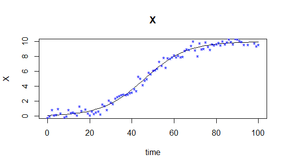
Subsequently, we can visualize the observations along the true solution of this simple ODE model as
#plot simulated data against generating model
plot(mod,ylab=names(state))      #curve
points(times, observ,pch='*',col='blue')    #observation
 First, a basis object needs to be defined by
 create.bspline.basis from fda package for smoothing observations. A B-spline basis is created given 21 konts including both interior and boundary knots acorss observation interval ((0,100)). The order of basis functions is 4, so there is a total of 23 basis functions.
#Generate basis object for interpolation and as argument of pcode
#21 konts equally spaced within [0,100]
knots <- seq(0,100,length.out=21)
#order of basis functions
norder <- 4
#number of basis funtions
nbasis <- length(knots) + norder - 2
#creating Bspline basis
basis  <- create.bspline.basis(c(0,100),nbasis,norder,breaks = knots)
To perform parameter cascade method for estimating both structural and nuisance parameters, one can use pcode in the following way
#parameter estimation
pcode.result <- pcode(data = observ, time = times, ode.model = ode.model,
                      par.initial = 0.3, par.names = 'theta',state.names = 'X',
                      basis.list = basis, lambda = 1e2)
The structural parameter and nuisance parameter estiamtes can be called by
pcode.result$structural.par
#>      theta
#> 0.09995229
pcode.result$nuisance.par
#>  [1]  0.1232160  0.1550332  0.1903906  0.2729993  0.4284428  0.6134020
#>  [7]  1.0222183  1.6891098  2.5351231  3.5543293  4.8116926  6.0699739
#> [13]  7.2145361  8.0734588  8.7456720  9.2110485  9.4866269  9.7101657
#> [19]  9.8736650  9.9650449 10.0098433  9.9950749  9.9846698
References
Ramsay, J. O., G. Hooker, D. Campbell, and J. Cao. 2007. “Parameter Estimation for Differential Equations: A Generalized Smoothing Approach.” Journal of the Royal Statistical Society. Series B (Statistical Methodology) 69 (5): 741–96.
 First, a basis object needs to be defined by