A bit of Theory

Manuel Chevalier

2022-07-01

The CREST method (Climate REconstruction SofTware) is a climate reconstruction technique that combines presence-only occurrence data with modern climatologies to estimate the conditional responses of a given set of taxa to a variable of interest [1-2]. The combination of these responses is used to estimate past climate probabilities. To illustrate the conceptual background of CREST, we will consider fossil pollen data, as these are great, ubiquitous climate proxies. One specific characteristic of pollen data is their limited taxonomical resolution. Usually, pollen cannot be identified at the species level but at a higher level (sub-genus to family level), which complexifies the modelling of the pollen-climate responses [3].

Defined as probability density functions (PDFs), these taxon-climate responses are estimated in one or two steps based on the nature of the proxy being studied. In simple cases, where fossils can be identified at the species level (e.g. foraminifers, plant macrofossils), the PDFs are defined by unimodal and parametric functions (e.g. normal or log-normal distributions depending on the nature of the studied variable, see [1-2] for a more detailed discussion). The parameters (e.g. 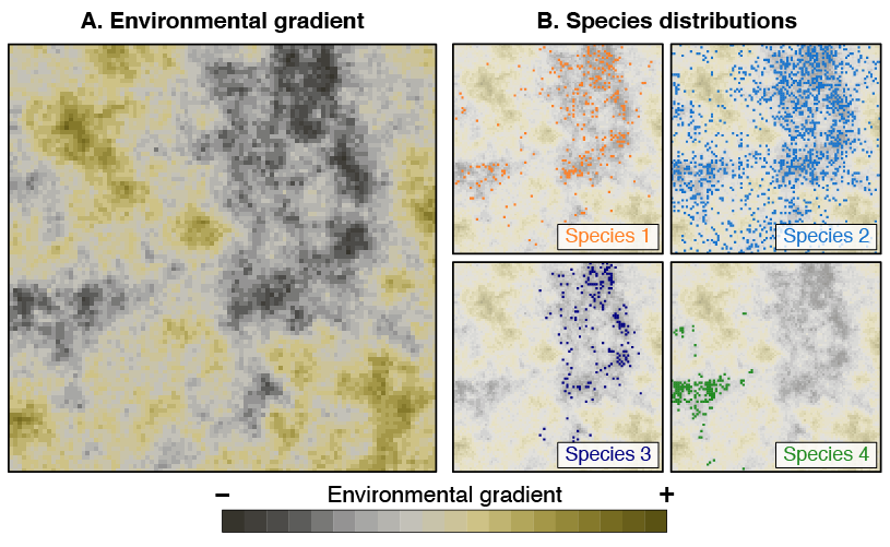a mean and a standard deviation in the case of a normal or log-normal distribution) describing these distributions are estimated from the ensemble of climate values corresponding to the presence records (Fig. 1), each being weighted as an inverse function of its abundance in the study area. This correction removes the influence of the heterogeneously distributed modern climate space and ensures that the optimum exhibited by the PDF reflects the true climatic preference of the species, rather than the modern abundance of a given climate value [4-5].

Fig. 1: (left) Climate variable to reconstruct (e.g. mean annual temperature). (Right) Four distinct plant taxa living in that region and having a preference for the darker climates (e.g. a preference for colder climates). These four species produce undistinguisable pollen grains and, therefore, define a ‘pollen type’. This example is based on pseudo-data.

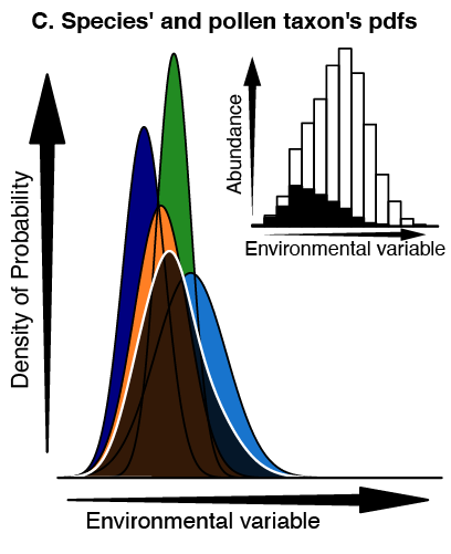
Two steps are necessary to create the taxon-climate probabilistic link when the fossils cannot be identified at the species level (e.g. pollen grains identified at the genus or family level). First, following the process above, a parametric PDF is created for each of the species producing the same type of pollen grains, and then, these PDFs are grouped together to create a higher-order PDF representing the pollen type, with each species being weighted as a function of the extent of its distribution (Fig. 2). One assumption of the model is that species with larger distributions are considered more likely to have produced the pollen grain observed in the absence of independent evidence. No additional assumptions are made concerning the shapes of these pollen PDFs, thus allowing them to be multimodal if different species/groupings exhibit different climate requirements. It is worth noting that the process can be used with incomplete distribution data because CREST uses parametric functions to define the species PDFs. Reconstructions from modern [1] and fossil [6-9] data suggest that robust PDFs can still be obtained from truncated geographical distributions, provided that the full range of the climatic tolerance of the species is well covered in the climate space [10].

Fig. 2: Climate responses of the four plant species presented on Fig. 1 (coloured curves). Their individual responses are combined together to create the response of the pollen taxon in black. The histogram inset represents the distribution of the climate space available (white) and which part of this climate space is occupied by at least one species (in black).

Finally, the PDFs for each fossil taxon identified in a sample are multiplied together, each with a weight derived from the observed percentages. Since relative abundances, different production rates and taphonomy are important factors influencing the fossil assemblage observed, direct percentages cannot be used directly, and they need to be transformed to minimise the effect of these factors. In CREST, the transformation is performed on a taxon basis by normalising the raw percentages by the average of the percentages of all the samples where the taxon is observed (i.e. the zeros are excluded). A value higher (lower) than one suggests that the climate at the time of deposition was more (less) favourable (i.e. 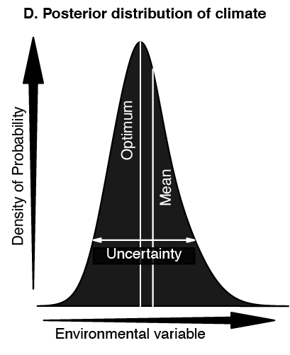closer to the taxon’s climate optimum) than the average climate in which the taxon has been observed during the studied period. The multiplication of PDFs results in a likelihood distribution along the climate gradient, from which climate estimates and uncertainties can be derived (Fig. 3). More technical details about the different parameterisations of the method can be obtained from the original publications (1-2).

Fig. 3: Likelihood distribution conditioned by the existence of certain fossil taxa observed with certain proportions. This distribution can be simplified to single number, such as the mean or the mode/optimum (i.e. the most likely) probability.

Compared to other existing climate reconstruction methods, the probabilistic nature of CREST also provides a unique opportunity to derive probabilistic reconstructions. Such likelihood distributions describe the likelihood of all the climate values along a studied climate gradient and not just a single ‘best estimate’ associated with a standard error [10]. The spread of these uncertainties represents the amount of information available for the studied system: well-constrained samples generally have relatively narrower uncertainty ranges than samples with fewer constraints. This advantage can ultimately be used in data-data comparisons and to assimilate CREST-based reconstructions with Earth System Models palaeo-simulations.

References

[1] Chevalier, M.,
Cheddadi, R., Chase, B.M., 2014. CREST (Climate REconstruction
SofTware): a probability density function (PDF)-based quantitative
climate reconstruction method. Clim. Past 10, 2081–2098. doi:10.5194/cp-10-2081-2014.
[2] Chevalier, M., 2022.
crestr an R package to perform probabilistic climate
reconstructions from palaeoecological datasets. Clim. Past doi:10.5194/cp-18-821-2022.
[3] Chevalier, M., 2019.
Enabling possibilities to quantify past climate from fossil assemblages
at a global scale. Global and Planetary Change, 175, pp. 27–35. doi:10.1016/j.earscirev.2020.103384.
[4] Kühl, N., Gebhardt, C.,
Litt, T., Hense, A., 2002. Probability Density Functions as
Botanical-Climatological Transfer Functions for Climate Reconstruction.
Quat. Res. 58, 381–392. doi:10.1006/qres.2002.2380.
[5] Bray, P.J., Blockley,
S.P.E., Coope, G.R., Dadswell, L.F., Elias, S.A., Lowe, J.J., Pollard,
A.M., 2006. Refining mutual climatic range (MCR) quantitative estimates
of palaeotemperature using ubiquity analysis. Quat. Sci. Rev. 25,
1865–1876. doi:10.1016/j.quascirev.2006.01.023.
[6] Chevalier, M., Chase, B.M.,
2015. Southeast African records reveal a coherent shift from high- to
low-latitude forcing mechanisms along the east African margin across
last glacial–interglacial transition. Quat. Sci. Rev. 125, 117–130. doi:10.1016/j.quascirev.2015.07.009.
[7] Chevalier, M., Chase, B.M.,
2016. Determining the drivers of long-term aridity variability: a
southern African case study. J. Quat. Sci. 31, 143–151. doi:10.1002/jqs.2850.
[8] Lim, S., Chase, B.M.,
Chevalier, M., Reimer, P.J., 2016. 50,000 years of climate in the Namib
Desert, Pella, South Africa. Palaeogeogr. Palaeoclimatol. Palaeoecol.
451, 197–209. doi:10.1016/j.palaeo.2016.03.001.
[9] Cordova, C.E., Scott,
L., Chase, B.M., Chevalier, M., 2017. Late Pleistocene-Holocene
vegetation and climate change in the Middle Kalahari, Lake Ngami,
Botswana. Quat. Sci. Rev. 171, 199–215. doi:10.1016/j.quascirev.2017.06.036.
[10] Chevalier, M.,
Davis, B.A.S., Heiri, O., Seppä, H., Chase, B.M., Gajewski, K.,
Lacourse, T., Telford, R.J., Finsinger, W., Guiot, J., Kühl, N.,
Maezumi, S.Y., Tipton, J.R., Carter, V.A., Brussel, T., Phelps, L.N.,
Dawson, A., Zanon, M., Vallé, F., Nolan, C., Mauri, A., de Vernal, A.,
Izumi, K., Holmström, L., Marsicek, J., Goring, S., Sommer, P.S.,
Chaput, M. and Kupriyanov, D., 2020. Pollen-based climate reconstruction
techniques for late Quaternary studies. Earth-Science Reviews, 210,
pp. 103384. doi:10.1016/j.earscirev.2020.103384.